How to Strikethrough in Excel: 7 Methods That Actually Work
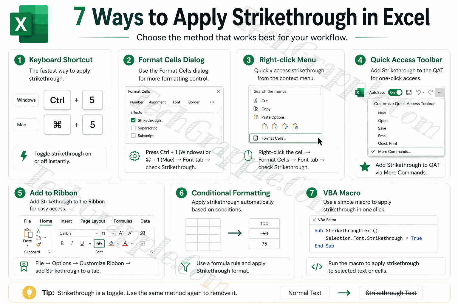
Strikethrough is one of those formatting options that Excel tucks away. It’s not sitting there on the ribbon like Bold or Italic. But once you know where to look — or which shortcut to press — it takes less than two seconds to apply.
Whether you’re marking tasks as done, crossing out outdated prices, or setting up a to-do tracker that automatically strikes through completed items, this guide covers the practical options for Excel on Windows, Mac, and the web.
Keyboard Shortcut and Excel for the Web
If you’re using desktop Excel, the keyboard shortcut is the fastest method. If you’re using Excel for the web, the Home tab’s Strikethrough button is the most reliable option because browser shortcuts can vary.
Windows desktop
Ctrl + 5
Standard shortcut in Excel for Windows
Mac desktop
⌘ Cmd + Shift + X
Common shortcut in Excel for Mac; Cmd + 5 also works in some setups
Excel for the web
Home → Strikethrough
Use the Font group if a browser shortcut does not work
How to Use It
- Select the cell or range you want to strikethrough.
- Press Ctrl + 5 on Windows, or ⌘ Cmd + Shift + X on Mac. If ⌘ Cmd + 5 works in your Mac or web setup, you can use that too.
- The strikethrough formatting is applied immediately. Use the same command again to remove it.
Excel for the web
In Excel for the web, select the cells, go to Home, then choose Strikethrough in the Font group. Some browser and keyboard combinations also support shortcuts such as Ctrl + 5 on Windows or ⌘ Cmd + 5 on Mac, but the ribbon button is the most reliable web method.
Ctrl + 5 applies strikethrough to the selected cell instantly
Pro Tip
You can apply strikethrough to multiple non-adjacent cells at once. Hold Ctrl on Windows or ⌘ Cmd on Mac while selecting the cells, then apply strikethrough. All selected cells get formatted in one go.
Format Cells Dialog Box
This is the most reliable desktop Excel method when you want to confirm exactly which font effects are applied. Strikethrough lives inside the Format Cells dialog, under the Font tab.
- Select the cell or range of cells you want to format.
- Press Ctrl + 1 to open the Format Cells dialog. (On Mac, use ⌘ Cmd + 1)
- Click the Font tab at the top of the dialog.
- Under the Effects section, check the box next to Strikethrough.
- Click OK to apply.
The Format Cells dialog — Font tab → Effects → Strikethrough checkbox
Shortcut to Open the Dialog
Instead of going to the ribbon, press Ctrl + 1 on Windows or ⌘ Cmd + 1 on Mac to open Format Cells directly.
Right-Click Context Menu
This method is a mouse-friendly version of Method 2 in desktop Excel. If you don’t remember the keyboard shortcut for Format Cells, right-clicking is the next quickest option.
- Select the cell or cells you want to apply strikethrough to.
- Right-click on the selection to open the context menu.
- Click Format Cells at the bottom of the menu.
- In the dialog that opens, click the Font tab.
- Under Effects, check the Strikethrough box, then click OK.
Right-click → Format Cells → Font tab → Strikethrough
Once the Format Cells dialog opens, the steps are identical to Method 2. Go to the Font tab, find the Strikethrough checkbox, tick it, and click OK.
Quick Access Toolbar (One-Click Strikethrough Button)
The Quick Access Toolbar (QAT) sits at the very top of the desktop Excel window. You can add a Strikethrough button there so it’s always one click away, no matter which tab you’re on.
You only need to set this up once. After that, it’s genuinely the most convenient option.
How to Add Strikethrough to the QAT
- Click the small dropdown arrow at the end of the Quick Access Toolbar (it looks like a downward chevron ⌄).
- Select More Commands at the bottom of the dropdown.
- In the “Choose commands from” dropdown, select Commands Not in the Ribbon.
- Scroll down the list until you find Strikethrough. Click on it to select it.
- Click the Add >> button to move it to the right panel.
- Click OK. The Strikethrough button now appears in your Quick Access Toolbar.
The Strikethrough button added to the Quick Access Toolbar — always visible at the top
Tip
You can also move the QAT below the ribbon if you prefer it closer to your data. Just click the dropdown arrow and choose Show Below the Ribbon.
Adding Strikethrough to the Home Ribbon
If you’d rather have Strikethrough in the main desktop ribbon rather than the QAT, you can add it there too. This requires creating a custom group on the Home tab.
- Right-click anywhere on the ribbon and choose Customize the Ribbon.
- In the right panel, select the Home tab and click New Group at the bottom. You can rename it something like “My Formatting”.
- In the left panel, change the “Choose commands from” dropdown to Commands Not in the Ribbon.
- Find Strikethrough in the list, select it, and click Add.
- Click OK. The button will appear in your new group on the Home tab.
Customize the Ribbon dialog — adding Strikethrough to a custom group in the Home tab
Note
Excel doesn’t let you add buttons to its built-in groups (like the Font group). You have to create a new custom group first, then add Strikethrough to that group.
Conditional Formatting — Automatic Strikethrough
This is where things get really useful. Conditional Formatting lets Excel automatically apply strikethrough when a certain condition is met — like when a task is marked “Done” or a checkbox is ticked.
Imagine a task list where you just change a cell to “Done” and the text in that row automatically crosses itself out. That’s exactly what this does.
Example: Strikethrough When Status is “Done”
Let’s say Column A has task names and Column B has the status (either “Done” or “Pending”). You can apply the rule to only the task names, or to the wider row if you want the due date and other related cells crossed out too.
- Select the cells you want Excel to cross out. Use A2:A20 for task names only, or a wider range such as A2:C20 if you want the row formatting to follow the status.
- Go to the Home tab → click Conditional Formatting → select New Rule.
- Choose “Use a formula to determine which cells to format”.
- Enter this formula in the formula box:
=$B2="Done" - Click the Format button. Go to the Font tab, check the Strikethrough box, and click OK.
- Click OK again to close the New Rule dialog.
Conditional Formatting: cells in rows marked “Done” get strikethrough applied automatically
Works With Checkboxes Too
If your status column uses checkboxes, set the formula to =$B2=TRUE. Checking the box will automatically apply the strikethrough.
VBA Macro — For Power Users
If you use strikethrough a lot and want ultimate control, you can write a simple VBA macro to apply or toggle it. This is especially useful when you want to trigger it via a button or as part of a larger automation.
Don’t be put off by “VBA” — the code here is short and simple.
How to Open the VBA Editor
- Press Alt + F11 on Windows, or Option + F11 on Mac, to open the Visual Basic Editor.
- In the left panel, double-click on Module1 (or insert a new module via Insert → Module).
- Paste the macro code below into the editor.
- Press F5 or choose the editor’s Run command to run it, or close the editor and assign it to a button.
Macro 1 — Apply Strikethrough to Selected Cells
Sub ApplyStrikethrough()
    ' Applies strikethrough to all selected cells
    Selection.Font.Strikethrough = True
End Sub
Macro 2 — Toggle Strikethrough On and Off
This version is smarter. It checks the current state and flips it — just like the keyboard shortcut does.
Sub ToggleStrikethrough()
    ' Toggles strikethrough on the current selection
    With Selection.Font
        .Strikethrough = Not .Strikethrough
    End With
End Sub
Macro 3 — Auto Strikethrough Based on Cell Value
This macro loops through a column and applies strikethrough to any row where the status cell says “Done”. Great for batch processing an existing list.
Sub StrikethroughDoneTasks()
    Dim ws As Worksheet
    Dim i As Long
    Dim lastRow As Long

    Set ws = ActiveSheet
    lastRow = ws.Cells(ws.Rows.Count, "B").End(xlUp).Row

    For i = 2 To lastRow  ' Start from row 2 (skip header)
        If ws.Cells(i, 2).Value = "Done" Then
            ws.Cells(i, 1).Font.Strikethrough = True
        Else
            ws.Cells(i, 1).Font.Strikethrough = False
        End If
    Next i
End Sub
Important
Files containing macros must be saved as .xlsm (Excel Macro-Enabled Workbook), not the regular .xlsx format. VBA macros are for desktop Excel, not Excel for the web.
All 7 Methods at a Glance
Not sure which method is right for your situation? Here’s a quick comparison.
| # | Method | Speed | Skill Level | Best For |
|---|---|---|---|---|
| 1 | Keyboard Shortcut / Web Button | Instant | Beginner | Everyday use in desktop Excel and Excel for the web |
| 2 | Format Cells Dialog | ~5 seconds | Beginner | Desktop Excel when combining multiple font changes |
| 3 | Right-Click Context Menu | ~6 seconds | Beginner | Mouse-only workflows in desktop Excel |
| 4 | Quick Access Toolbar | Instant (after setup) | Beginner | Regular desktop use, one-click access |
| 5 | Custom Ribbon Button | Instant (after setup) | Intermediate | Desktop users who prefer the ribbon over QAT |
| 6 | Conditional Formatting | Automatic | Intermediate | To-do lists, task trackers, dashboards |
| 7 | VBA Macro | Instant (after setup) | Advanced | Desktop automation, batch processing, custom buttons |
Bonus: Strikethrough on Part of a Cell’s Text
Most Excel strikethrough workflows apply the formatting to the entire cell. But what if you only want to cross out part of the text — like changing a price from $299 to $199?
Here’s how to do it:
- Double-click the cell to enter edit mode, or click once in the formula bar.
- Use your mouse or keyboard to select just the part of the text you want to cross out.
- Press Ctrl + 1 on Windows or ⌘ Cmd + 1 on Mac to open Format Cells. You can also right-click the selected text and choose Format Cells in desktop Excel.
- On the Font tab, check Strikethrough and click OK.
Note
For partial text formatting, use the Format Cells dialog or the Font controls while editing inside the cell. The basic keyboard shortcut is best for formatting complete cells.
How to Remove Strikethrough in Excel
Removing strikethrough is just as easy as applying it. Use the same method you used to add it:
- If you used the keyboard shortcut, press the same shortcut again. On Windows, that is usually Ctrl + 5. On Mac, use the shortcut that worked for your Excel version.
- If you used Format Cells, open it again, uncheck the Strikethrough box, and click OK.
- If you used Excel for the web, select the cells and choose Home → Strikethrough again.
- If it was applied via Conditional Formatting, you’ll need to edit or delete that rule. Just go to Home → Conditional Formatting → Manage Rules.
You can also clear all formatting from a cell by going to Home → Clear → Clear Formats. Just note that this removes all formatting — not just the strikethrough.
Quick Recap
Strikethrough in Excel isn’t hard once you know where to find it. Here’s what to take away:
- Fastest desktop method: Ctrl + 5 on Windows, or ⌘ Cmd + Shift + X on Mac. ⌘ Cmd + 5 may also work depending on your Mac or browser setup.
- Best web method: Home → Strikethrough in Excel for the web. Browser shortcuts vary, but the ribbon button is reliable.
- Most accessible desktop method: Format Cells dialog (Ctrl+1 or Cmd+1 → Font tab → Strikethrough).
- Best for convenience: Add a Strikethrough button to your Quick Access Toolbar — a one-time setup that saves time forever.
- Most powerful: Conditional Formatting for dynamic, automatic strikethrough based on cell values.
- For automation: A simple VBA macro gives you full control and flexibility.
There’s no single “best” method — it depends on whether you’re using desktop Excel, Excel for the web, or building an automated workflow.